by Ivan Vankov
Share
by Ivan Vankov

Search is an important capability in computer science with numerous practical applications. People use search technologies every day when using popular websites and search engines. Full-text search has been around for a long time, and with the emerging importance of AI vector search, full-text search is now becoming more relevant. In this article, we compare a traditional full-text search to a vector search using a PostgreSQL instance in a cloud environment.
Introduction
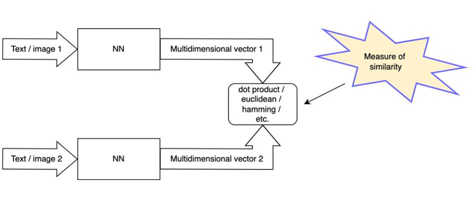
Vector search is a method of searching and ranking results based on conversion of a search query into a vector representation and comparing it against vector representations of searched documents. The closer the vector of a document to the vector of the query, the more relevant it is.
Multiple measures of proximity exist, including Euclidean distance, inner product, or cosine distance.
To generate vectors (also called embeddings) a neural network model is used.
Vectors and corresponding documents are stored in a vector store. Because the number of documents can be large vector stores, implement indexing techniques to speed up the search for relevant results. To name few:
- Locality-Sensitive Hashing (LSH)
- Inverted File Index (IVF)
- Hierarchical Navigable Small World (HNSW)
- Product Quantization (PQ), Scalar Quantization (SQ)
- Composite methods, e.g. HNSW_SQ, IVF_PQ
Pgvector is an extension that provides vector store capabilities in PostgreSQL. Pgvector uses HNSW (Hierarchical Navigable Small World) graph for indexing. HNSW is a multilayer graph that operates like a probabilistic data structure skip-list. Each node in the graph is a vector while edges connect the nodes that are close to each other. Search is performed by descending from the higher layer to the layer 0 and performing breadth-first search at each layer to find the closest matching vectors.
Full-text search uses variations of TF-IDF (Term Frequency–Inverse Document Frequency), word stemming, lists of stop words, synonym dictionaries, and may use some other rule-based algorithms. The inverted index is used to improve search performance, i.e. a mapping from word to the list of documents in which the word appears along with some additional information.
PostgreSQL provides GIN (Generalized Inverted Index) and GiST (Generalized Search Tree) index types and several operations for full-text search. Built-in ranking functions consider how often the query terms appear in the document, how close together the terms are in the document, and how important the part of the document where they occur is.
Playground Setup
In this section a setup of PostgreSQL playground in Google Cloud is briefly described to measure indexes performance. The next section provides the results of the comparison.
We set up the PostgreSQL instance using Cloud SQL. The PostgreSQL Cloud SQL instance includes pgvector extension by default. We will only need to enable it with a simple SQL statement.
For embeddings generation for both indexed documents and search queries textembedding-gecko@001 model was used following the example. Using this notebook with a small modification in the step “Save the embeddings in JSON format” that includes the questions title and body in the output JSON we can generate JSON files with the following structure:
“`json[
{
“id”: 1,
“embedding”: [0.123456789, 0.123456789, …, 0.123456789],
“text”: “Question 1 header\nQuestion 1 content”
},
{
“id”: 2,
“embedding”: [0.234567891, 0.234567891, …, 0.234567891],
“text”: “Question 2 header\nQuestion 2 content”
},
…
]
“`
Create Cloud SQL instance (replace value of DB_PASS with an arbitrary password when you run it):
“`shell
DB_USER=postgres
DB_PASS=[password]
MY_PUBLIC_IP=$(curl ipinfo.io/ip)
gcloud auth login
gcloud sql instances create search-test \
–authorized-networks=${MY_PUBLIC_IP} \
–availability-type=ZONAL \
–root-password=”${DB_PASS}” \
–storage-auto-increase \
–storage-size=10G \
–region=”us-central1″ \
–tier=”db-custom-2-8192″ \
–database-version=POSTGRES_15
“`
Note, that the connection to the instance is allowed only from the public IP that is defined by variable MY_PUBLIC_IP.
After the instance becomes available, we connect to it using a PostgreSQL client and public IP or Cloud SQL Studio in Google cloud console. There we enable vector extension and create a table and indexes for the vector and for the full-text search:
After the instance becomes available, we connect to it using a PostgreSQL client and public IP or Cloud SQL Studio in Google cloud console. There we enable vector extension and create a table and indexes for the vector and for the full-text search:
“`SQL
CREATE EXTENSION IF NOT EXISTS vector;
CREATE TABLE IF NOT EXISTS question_store (
id integer primary key,
embedding vector(768),
content text
);
CREATE INDEX IF NOT EXISTS hnsw_l2 ON question_store USING HNSW (embedding vector_l2_ops);
CREATE INDEX IF NOT EXISTS search_idx ON question_store USING GIN (to_tsvector(‘english‘, content));
“`
Next, load data in PostgreSQL. Install package psycopg2 if necessary, and update variables in the beginning of the script: specify public IP of Cloud SQL instance as value for HOST variable (the IP address can be found in the details of the instance in Google cloud console), specify the password as value of PASS variable, and update value of FILE_NAME_PREFIX accordingly. Also, to avoid connection issues make sure to run the script from the machine whose public IP was specified when SQL instance was created. You can add additional allowed public IPs in the Cloud SQL instance settings in Google Cloud console:
“`python
import psycopg2
import json
HOST=” 34.67.204.142″
DB=“postgres”
USER=“postgres”
PASS=“”
FILE_NAME_PREFIX=“/tmp/tmp5o9ucvho/tmp5o9ucvho_”
connection = psycopg2.connect(database=DB, user=USER, password=PASS, host=HOST, port=5432)
cursor = connection.cursor()
def load_vectors(i: int):
result = []
with open(FILE_NAME_PREFIX + str(i) + “.json”, “r”) as vectors:
line = vectors.readline()
while len(line) > 0:
result.append(json.loads(line))
line = vectors.readline()
return result
def do_upload(i: int):
entries = load_vectors(i)
print (“loading “ + str(len(entries)) + ” entries”)
args_str = “”
for entry in entries:
id = int(entry[“id”])
content = entry[“text”]
embedding = str(entry[“embedding”]).replace(“‘”, “”)
args_str += cursor.mogrify(“(%s,%s,%s)”, (str(id), embedding, content)).decode(“utf-8”)
args_str += “,”
cursor.execute(“insert into question_store(id, embedding, content) values” + args_str.rstrip(‘,’))
connection.commit()
print(“done “ + str(i))
for i in range(0, 10):
do_upload(i)
print(“finished”)
connection.close()
“`
The script will upload the data in several batches. In the beginning it imports required packages, defines variables, then opens a connection to PostgreSQL and starts a transaction. The function load_vectors() reads the previously generated data in JSON format from files at location defined by the global variable FILE_NAME_PREFIX, e.g. /tmp/tmp5o9ucvho/tmp5o9ucvho_0.json, /tmp/tmp5o9ucvho/tmp5o9ucvho_1.json, etc. The function do_upload() reads the JSON file and prepares an insert SQL statement with the embeddings and then executes it and commits the transaction. Finally, the script goes through 10 iterations (one iteration per file) each time calling do_upload().
To select top 5 Stack Overflow questions most relevant to your query you can use the SQL statements:
“`SQL
SELECT content, embedding <-> ‘[1,2,3]’ AS distance FROM question_store WHERE embedding <-> ‘[1,2,3]’ < 1 ORDER BY distance LIMIT 5;
SELECT id, content FROM (SELECT id, content, ts_rank_cd(to_tsvector(‘english‘, content), query) AS rank FROM question_store, to_tsquery(”) query WHERE query @@ to_tsvector(‘english‘, content) ORDER BY rank DESC LIMIT 5) as t
“`
The first statement uses vector search and HNSW index. Relevant vectors can be generated from the search query text using the previously mentioned model textembedding-gecko@001 by calling function encode_texts_to_embeddings() defined in the notebook (which should not be a problem if you made it to this point).
The second statement uses full-text search using the search query text directly specified in the statement as “”.
Results and Conclusion
Using system view pg_stat_statements and functions pg_relation_size, pg_total_relation_size we can extract information about the execution speed and the size of full-text search and vector search:
| Name | Values |
|---|---|
| Number of rows | 50000 |
| Table size with indexes | 489 MB |
| HNSW index size | 195 MB |
| GIN index size | 40 MB |
| Type | min_exec_time (ms) | max_exec_time (ms) | mean_exec_time (ms) |
|---|---|---|---|
| Vector (HNSW) | 2.4 | 5.0 | 3.4 |
| Full-text (GIN) | 1.4 | 871.9 | 101.2 |
As we can see the HNSW index is 2.5 times larger than GIN index for the same data. Full-text search has higher variance in query time. It is slower on average, but we need to consider that to perform vector searches, we also need to generate embeddings from the text query. It takes about 100ms to generate one vector using API call to textembedding-gecko@001 in the same region where the model is hosted.
From a qualitative point of view full-text search is more rigid and beneficial for finding exact matches and terms, while vector search is more suitable for searching by meaning. Also, vector search better handles grammatical mistakes in the search query.
Taking the resource consumption in proportion to the full CPU and disk capacity, the estimated cost of 10,000 vector search request per day with average length of 100 characters per request is about $2.00 including the cost of API calls for embeddings generation. While for full-text search with similar characteristics the price is less than $1. Google Cloud’s pricing calculator can be used to estimate the cost.
If you followed the steps for creating the playground don’t forget to tear down the Cloud SQL instance and clean up other resources that you may have allocated in GCP.